AE Data
Accessing Data
Overview
The source climate projections produced for California’s Fifth Climate Change Assessment that underlie the Cal-Adapt: Analytics Engine are freely available and accessible to the public. The projections can be accessed through Amazon’s Registry of Open Data and are hosted on Amazon Web Services (AWS) as part of the data catalog for the Cal-Adapt: Analytics Engine’s “Co-Produced Climate Data to Support California’s Resilience Investments.”
The Open Data program democratizes access by making data publicly available, enabling the use of cloud-optimized datasets, techniques, and tools in cloud-native formats, and building communities that benefit from these shared datasets. Because the Analytics Engine is part of the Open Data program, all climate projections are accessible now.
The Analytics Engine hosts nearly 1 petabyte (1000 terabytes) of multi-dimensional array data, and the size and complexity of this data make it important to become familiar with the structure of the data before trying to access or download.
Data Structure and Format
The Analytics Engine public AWS S3 bucket named cadcat, short for Cal-Adapt: Data Catalog, contains dynamically downscaled WRF data in Zarr and statistically downscaled LOCA2-hybrid data in both NetCDF and Zarr formats, along with other datasets such as station data (HadISD). More detailed information about the climate data used by the Cal-Adapt: Analytics Engine can be found in the About the Data section.
NetCDF Files
The raw LOCA2-Hybrid datasets are stored as NetCDF files in S3 at the subdirectory LOCA2/aaa-ca-hybrid. The advantage of NetCDF files is that they are single files stored in a directory structure, and can thus be manually downloaded using a web browser for a minimal set of data. The disadvantage of NetCDF is that they need to be loaded completely into memory to access even a slice of the data, which can be resource exhaustive or even prohibitive.
Zarr Stores
The majority of the climate data for the Cal-Adapt: Analytics Engine stored on AWS S3 is in a cloud-optimized multi-dimensional array format known as Zarr. Zarr stores can be randomly accessed to retrieve a slice of the data and do not require that the entire dataset be loaded into memory. This is vitally important when dealing with hourly data over large spatial and temporal extents. The Zarrs are stored in S3 in a hierarchical directory structure designed to work in conjunction with Intake ESM to make the data discoverable, searchable, and easier to access. The directory structure is prescribed by the Intake ESM system and can be non-intuitive to users not familiar with it. Zarr stores have many directory levels, which make it difficult to download manually using a web browser. Either the use of AWS’s command line interface (AWS CLI) for S3 or Python programming is needed to access and/or download the data in this format. A web browser can be helpful in understanding the data structure before attempting to access specific files. AWS allows users to browse S3 buckets via a web browser - here is the top level of the cadcat bucket AWS S3 Explorer.
There are 4 main collections of Zarr datasets in the S3 bucket:
- WRF - Dynamically-downscaled global climate models performed by the Weather Research and Forecasting model
- LOCA2-Hybrid - Statistically-downscaled global climate models performed by LOCA (Localized Constructed Analogs) version 2 for California
- HadISD - Hadley Centre observations datasets (station data). Does not conform to the Intake ESM data structure, and is not part of the Intake ESM data catalog.
- HistWxStns - Historical observation datasets (station data), including the HadISD stations.
WRF and LOCA2-Hybrid follow similar directory structures with some notable differences:
- LOCA2-Hybrid has an additional level (Variant/member_id)
- Not all parameters are the same between WRF and LOCA2-Hybrid
- Parameters are not always internally consistent.
More advanced query tools are useful in figuring out where the data is and how to load it into different software packages. The Analytics Engine searchable Data Catalog was generated from the contents of the Intake ESM catalog to help identify the exact path to the data of interest. Users can type into the search box to identify datasets of interest and view the path to those datasets in the S3 bucket structure.
How can users access, visualize, and download climate data from the Analytics Engine?
Once a user has identified a specific dataset of interest, there are many ways to access, visualize, and download that data from the Analytics Engine (AE). A variety of ways to access the Analytics Engine data are detailed below:
Cal-Adapt: Analytics Engine JupyterHub
Energy-sector users with a Cal-Adapt: Analytics Engine JupyterHub login can access co-produced, pre-developed Jupyter notebooks to analyze, subset, and utilize existing Cal-Adapt: Analytics Engine data. The code and data can be customized for individual needs through the JupyterHub web interface, which provides private cloud storage through Amazon Web Services. Users can then export data in a variety of formats to cloud storage or a local machine. This solution requires a Cal-Adapt: Analytics Engine login, although all the Analytics Engine notebook code is open source and publicly available via our cae-notebooks GitHub repository.
Best Use
The Analytics Engine JupyterHub is currently exclusively provided to energy-sector partners in California, in alignment with funding from the California Energy Commission. The JupyterHub environment is hosted in AWS and has access to cluster processing, 32GB of RAM, 10GB of storage on the Hub instance, and access to S3 storage for exporting larger datasets. It can be used to do any data processing on the Analytics Engine of interest.
Limitations
Not yet accessible to the general public. Limited to the resources provided by the HUB instance.
Example Usage
To support a range of workflows, the Analytics Engine provides data access notebooks that demonstrate various methods, including direct code-based access using climakitae, an intuitive graphical user interface (GUI) using the add-on package, climakitaegui, and options for accessing data outside of the Analytics Engine environment.
Running the Analytics Engine in Your Organization’s cloud
Organizations that require their own dedicated computing environment can deploy the Analytics Engine within their own AWS cloud infrastructure. This is done using a Docker image from the Pangeo team, which is run in a container via Kubernetes with JupyterHub on AWS EKS (Elastic Kubernetes Service). This approach is best suited for organizations with AWS cloud infrastructure and technical staff familiar with containerized environments.
Resources to get started:
- Instructions on setting up the Analytics Engine
- Resources on working in Docker environments
- Deploying JupyterHub on Kubernetes
Best Use
Organizations with AWS cloud infrastructure that need to run Analytics Engine workflows at scale within their own environment, maintain data privacy, or integrate Analytics Engine tools with internal data and systems.
Limitations
Requires organizational AWS infrastructure and familiarity with Docker and Kubernetes. Setup and maintenance are the responsibility of the deploying organization rather than the Analytics Engine team.
Accessing or downloading data using the climakitae Python package
A powerful Python toolkit for climate data retrieval and analysis has been developed as part of the Analytics Engine project, climakitae. The main features of the toolset are:
- Comprehensive Climate Data Access: Retrieve climate variables from hosted climate models
- Downscaled Climate Models: Access dynamical (WRF) and statistical (LOCA2) downscaling methods
- Spatial Analysis Tools: Built-in support for geographic subsetting and spatial aggregation
- Climate Indices: Calculate heat indices, warming levels, and extreme event metrics
- Flexible Data Export: Export to NetCDF, CSV, and Zarr
- GUI Integration: Works seamlessly with
climakitaeguifor interactive analysis
climakitae includes built-in methods to aid in the retrieval of data from the cadcat S3 bucket that are more intuitive and user-friendly than using the Python intake package directly..
Best Use
Powerful functionality allows users to retrieve data by warming level, by spatial and/or temporal filtering, by spatial and/or temporal aggregation, by derived variable, or by concatenated timeseries for historical and future scenarios. Allows users to utilize all of the Analytics Engine software functionality contained within the Analytics Engine JupyterHUB, especially when combined with the notebooks developed for the HUB in the cae-notebooks repository.
Limitations
Limited to the resources on the local computer (RAM, CPU, network), dataset processed from the original (simulations and time series concatenated, metadata added, warming levels calculated.
Example Usage
Specifically, the get_data function allows users to specify filtering parameters to get just the information needed instead of entire datasets, which helps ease the data size limitations of CMIP6 data.
To get started, users will need to set up a conda Python environment (pip environments are possible but harder to setup) with the necessary Python libraries. This README was created to help set up the environment. The basic steps are installing conda, downloading a curated list of supporting libraries, creating a new environment with those, and then downloading and installing climakitae. Once setup in the conda environment, run Python and enter these commands:
from climakitae.core.data_interface import get_dataThis loads the get_data function from the package. The function has the following input parameters:
| Parameter | Description | Example |
|---|---|---|
| variable (required) | String name of climate variable | “Air temperature at 2m”, “Maximum air temperature”, etc. |
| resolution (required) | Resolution of data in kilometers | “3 km”, “9 km”, or “45 km” |
| timescale (required) | Temporal frequency of dataset | “hourly”, “daily”, or “monthly” |
| downscaling_method (required) | Downscaling method of the data | “Dynamical” (WRF), “Statistical” (LOCA2-Hybrid), “Dynamical+Statistical” (Both) |
| data_type | Whether to choose gridded data or weather station data | “Gridded”, or “Stations” |
| approach | Time based or Warming Level based | “Time”, or “Warming Level” |
| scenario | SSP scenario and/or historical data selection | “SSP 3-7.0”, “SSP 2-4.5”,“SSP 5-8.5” “Historical Climate”, “Historical Reconstruction” |
| units | Variable units | Defaults to native |
| area_subset | Area category | “CA counties” |
| cached_area | Area | “Alameda county” |
| area_average | Take an average over spatial domain? | “Yes”, or “No” |
| latitude | Tuple of valid latitude bounds | (32, 36) |
| longitude | Tuple of valid longitude bounds | (-132, -128) |
| time_slice | Time range for retrieved data | (2045, 2075) |
| stations | Which weather station to retrieve localized downscaled model data at | KSAC (Sacramento Airport) |
| warming_level | Must be one of the warming levels available in clmakitae.core.constants | |
| warming_level_window | Years around Global Warming Level (+/-) \n (e.g. 15 means a 30yr window) | |
| warming_level_months | Months of year for which to perform warming level computation | |
| all_touched | Spatial subset option for within or touching selection | True, or False |
| enable_hidden_vars | Return all variables, including the ones in which “show” is set to False? | True or False |
This list is exhaustive. Most analyses require only a small sub-set of these options. They are there to allow for the production of all the datasets needed for the Analytics Engine code and notebooks.
Another way to get the list of parameters just listed is to query the function documentation at the Python command line:
from climakitae.core.data_interface import get_data
print(get_data.__doc__)
A simple example of how to use this function is:
from climakitae.core.data_interface import get_data
data = get_data(
    variable="Air Temperature at 2m",
    downscaling_method="Dynamical",
    resolution="9 km",
    timescale="monthly",
    scenario="SSP 3-7.0",
    cached_area="CA"
)
This will retrieve the WRF Air Temperature (t2) variable as an xarray DataArray for scenario SSP 3-7.0, at 9 km resolution, and on a monthly timescale for the whole state of California. To help with analysis, the data is transformed somewhat, so if users are interested in the raw data then the AWS CLI, or intake methods are recommended. For a lookup table of variable names used by the get_data function, see Variable Descriptions.
There are a few helper functions that go along with get_data to help understand what is available to retrieve from the data store. The get_data_options function returns a pandas DataFrame (table object) of the data options:
from climakitae.core.data_interface import get_data_options
get_data_options()
The returned Pandas DataFrame contains the fields downscaling_method, scenario, timescale, variable, and resolution. It is very similar to the Data Catalog found on the Analytics Engine website.
Using the get_data_options function with no parameters returns the entire list of datasets. Users can specify optional parameters to query the data catalog and find a more refined set of data.
from climakitae.core.data_interface import get_data_options
get_data_options(
    downscaling_method = "Statistical", # LOCA2-Hybrid
    resolution = "3 km"
)
This will refine the returned DataFrame to only the datasets matching the criteria. As another example to specify daily precipitation datasets:
get_data_options(
    variable = "precipitation",  # not a variable name, but close
    timescale = "daily"
)
The “precipitation” string entered actually does not exactly match any variable name in the data catalog, but the command will provide this information and suggest closely matching variable names. It will also default to one of those variables and return values for it. This suggestion logic applies to the other queryable fields as well.
Another helper function, get_subsetting_options, is used to spatially subset the data retrieved. There is a separate data catalog that stores Adobe parquet geospatial files that store the geometries for states, CA counties, CA Electricity Demand Forecast Zones, CA Watersheds, CA Electric Balancing Authority Areas, CA Electric Load Serving Entities, and Stations. For example, to get a list of counties available, use this command:
from climakitae.core.data_interface import get_subsetting_options
get_subsetting_options(area_subset = "CA counties")
This returns a Pandas DataFrame containing a list of cached_area values that can be used to spatially filter results when using get_data.
Return to get_data and apply some of the knowledge gained by using the helper functions get_data_options and get_subsetting_options. The minimum required inputs to get_data are: variable, resolution, and timescale. Optionally, users can spatially subset with: area_subset, cached_area, and area_average (set to “Yes” to aggregate the data to the selected geometry). Additionally, users can set the downscaling method, approach (Time or Warming Level), scenario, units, time_slice, warming_level, warming_level_window, and/or warming_level_months.
As an example of a time-based approach, request monthly 3 km resolution statistically downscaled historical precipitation using the following command:
data = get_data(
    variable = "Precipitation (total)",
    downscaling_method = "Statistical", # LOCA2-Hybrid
    resolution = "3 km",
    timescale = "monthly",
    scenario = "Historical Climate"
    # approach = "Time" # Optional because "Time" is the function default
)
Apply a spatial filter simply by setting the cached_area parameter, and then calculate the area average by using the area_average parameter:
data = get_data(
    variable = "Precipitation (total)",
    downscaling_method = "Statistical",
    resolution = "3 km",
    timescale = "monthly",
    scenario = "Historical Climate",

    # Modify location settings
    cached_area = "San Bernardino County",
    area_average = "Yes"
)
Alternatively, to retrieve WRF precipitation for a specific time period and several scenarios:
data = get_data(
    variable = "Precipitation (total)",
    downscaling_method = "Dynamical", # WRF
    resolution = "45 km",
    timescale = "monthly",
    cached_area = "San Bernardino County",

    # Modify time-based settings
    time_slice = (2000,2050),
    scenario = [
        "Historical Climate",
        "SSP 3-7.0",
        "SSP 2-4.5",
        "SSP 5-8.5"
    ]
)
Now, retrieve the data at a warming level instead of using the time-based approach. By default the 2.0 warming level is returned:
get_data(
    variable = "Precipitation (total)",
    downscaling_method = "Dynamical",  # WRF
    resolution = "45 km",
    timescale = "monthly",
    cached_area = "San Bernardino County",

    # Modify your approach
    approach = "Warming Level",
)
By default, a window of +/- 15 years is used to determine the warming level data retrieved. To modify the time window for a 20-year window and retrieve specific warming levels, do the following:
data = get_data(
    variable = "Precipitation (total)",
    downscaling_method = "Dynamical",
    resolution = "45 km",
    timescale = "monthly",
    cached_area = "San Bernardino County",
    approach = "Warming Level",

    # Modify warming level settings
    warming_level_window = 10,
    warming_level = [2.5, 3.0, 4.0]
)
The get_data function by default retrieves gridded data, but users can retrieve dynamically-downscaled climate data at the unique grid cell(s) corresponding to a desired historical weather station(s) that has undergone additional localization (i.e., bias-adjustment) to that weather station.This data can be retrieved using the data_type and stations arguments. If the stations argument is not set, the function will return all available weather stations– a hefty data retrieval that takes a while to run and is not recommended. Localization of climate models for historical weather station data is only available for Air Temperature. To retrieve data for a single station:
data = get_data(
    variable = "Air Temperature at 2m", # Required argument
    resolution = "9 km", # Required argument. Options: "9 km" or "3 km"
    timescale = "hourly", # Required argument
    data_type = "Stations", # Required argument
    stations = "San Diego Lindbergh Field (KSAN)" # Optional argument
)
Here is a more complex retrieval that retrieves two stations for a five-year period and returns the data in degrees Fahrenheit instead of Celsius:
data = get_data(
    variable = "Air Temperature at 2m",
    resolution = "3 km",
    timescale = "hourly",
    data_type = "Stations",
    stations = [
        "San Francisco International Airport (KSFO)",
        "Oakland Metro International Airport (KOAK)",
    ],
    units = "degF",
    time_slice = (2000,2005)
)
Users can also retrieve localized station data for future scenarios. The following command retrieves both the historical and SSP 3-7.0 scenarios for the time period 2000-2035:
data = get_data(
    variable = "Air Temperature at 2m",
    resolution = "9 km",
    timescale = "hourly",
    data_type = "Stations",
    stations = "Sacramento Executive Airport (KSAC)",
    units = "degF",
    time_slice = (2000,2035),
    scenario = ["Historical Climate", "SSP 3-7.0"]
)
Upon data retrieval, the historical and future SSP data are combined into a single timeseries for ease of use, rather than two separate data objects representing each time period individually. The localization procedure uses the historical weather station data to accurately bias-adjust the historical period, which is then applied to the SSP data.
To export (save the data to local storage) the DataArray returned by get_data, use either the xarray export functions or climakitae, which includes a built-in export function that handles metadata and formatting issues. The S3 saving option is reserved for users of the Analytics Engine JupyterHUB. Data can be exported to NetCDF, Zarr, or CSV. The climakitae export function will also inform the user when the data is very large or will fill up the drive that is targeted. Here is a sample workflow for exporting using climakitae:
import climakitae as ck
# NetCDF4 export locally
ck.export(data, filename="my_filename1", format="NetCDF")
# Zarr export locally
ck.export(data, filename="my_filename2", format="Zarr")
# CSV export locally
ck.export(data, filename="my_filename4", format="CSV")
Accessing or downloading data using Python intake package
As part of building climakitae, we created an intake data catalog, that allows for easy programmatic access to the data used on the Cal-Adapt: Analytics Engine, and is specifically an implementation of intake-ESM, which is designed for climate data. This catalog can be opened using Python by knowing the URL of the catalog file.
Best Use
Accessing the cae-collection of data in Python without having to download the dataset completely. Allows for spatial and temporal filtering of the data before exporting to the local filesystem. It can also be used to analyze large datasets with xarray and dask, and to convert the data to NetCDF if there is sufficient memory.
Limitations
Can only help access data that is in the cae-collection intake catalog. Other datasets in the cadcat S3 bucket have to be referenced manually using this option. To access all the data in the bucket, look into using the next option, the climakitae python package.
Example Usage
First, install the prerequisites:
pip install intake-esm==2023.11.10 s3fsThen open the intake-esm data catalog for querying:
import intake
cat = intake.open_esm_datastore(
'https://cadcat.s3.amazonaws.com/cae-collection.json'
)
This json file stores all the metadata and paths to the data contained in the catalog and populates the intake database. To see the unique attributes contained in the catalog, run:
cat.unique()

# code output
activity_id                                                 [LOCA2, WRF]
institution_id                                         [UCSD, CAE, UCLA]
source_id              [ACCESS-CM2, CESM2-LENS, CNRM-ESM2-1, EC-Earth...
experiment_id           [historical, ssp245, ssp370, ssp585, reanalysis]
member_id              [r1i1p1f1, r2i1p1f1, r3i1p1f1, r10i1p1f1, r4i1...
table_id                                          [day, mon, yrmax, 1hr]
variable_id            [hursmax, hursmin, huss, pr, rsds, tasmax, tas...
grid_label                                               [d03, d01, d02]
path                   [s3://cadcat/loca2/ucsd/access-cm2/historical/...
derived_variable_id                                                   []
The parameters on the left should look familiar from the discussion of the data directory structure at the beginning of this primer. Here is a table that describes what these parameters mean:
| Familiar Name | CMIP6 Term |
|---|---|
| Downscaling Method | activity_id |
| Institution | institution_id |
| Source | source_id |
| Experiment | experiment_id |
| Variant | member_id |
| Frequency | table_id |
| Variable | variable_id |
| Resolution | grid_label |
The intake-esm catalog can be filtered using the search method:
cat_subset = cat.search(activity_id="LOCA2")
cat_subset.unique()

# code output
activity_id                                                      [LOCA2]
institution_id                                                    [UCSD]
source_id              [ACCESS-CM2, CESM2-LENS, CNRM-ESM2-1, EC-Earth...
experiment_id                       [historical, ssp245, ssp370, ssp585]
member_id              [r1i1p1f1, r2i1p1f1, r3i1p1f1, r10i1p1f1, r4i1...
table_id                                               [day, mon, yrmax]
variable_id            [hursmax, hursmin, huss, pr, rsds, tasmax, tas...
grid_label                                                         [d03]
path                   [s3://cadcat/loca2/ucsd/access-cm2/historical/...
derived_variable_id                                                   []

cat_subset.unique()['source_id']

['ACCESS-CM2', 'CESM2-LENS', 'CNRM-ESM2-1', 'EC-Earth3', 'EC-Earth3-Veg', 'FGOALS-g3', 'GFDL-ESM4', 'HadGEM3-GC31-LL', 'INM-CM5-0', 'IPSL-CM6A-LR', 'KACE-1-0-G', 'MIROC6', 'MPI-ESM1-2-HR', 'MRI-ESM2-0', 'TaiESM1']
Further refinement of the catalog search supports finding a particular dataset using the available attributes (not all combinations are possible). The AWS S3 Explorer and the Data Catalog are useful for figuring out needed attributes:
cat_1model = cat.search(
activity_id="LOCA2",
source_id="ACCESS-CM2",
experiment_id="historical",
member_id="r1i1p1f1",
table_id="mon",
variable_id="tasmax"
)
This will narrow the catalog records to just one dataset. From there, these commands may be used to load the dataset:
dset_dict = cat_1model.to_dataset_dict(zarr_kwargs={'consolidated': True}, storage_options={'anon': True})
ds = dset_dict['LOCA2.UCSD.ACCESS-CM2.historical.mon.d03']
Intake returns a dictionary of xarray datasets so that the catalog query may be used to return multiple datasets (such as getting historical and SSP’s, or all models). In this case we have just one dataset and can pull it out of the dictionary and assign it to an object of its own. This object is a reference to the data, not the data itself. It can now be used to further filter and/or reshape the data if desired. To save the dataset as a NetCDF file, run this command:
ds.to_netcdf('LOCA2_UCSD_ACCESS-CM2_historical_mon_d03.nc', encoding={k: {'zlib': True, 'complevel': 6} for k in ds})Reading the catalog CSV and Zarrs from multiple languages
The Intake-ESM Catalog CSV file can be parsed and searched directly from many programming languages in addition to Python. From there, any of the datasets can be opened using languages with a Zarr implementation, of which there are many to choose from.
Best Use
Programmatic access from multiple languages with a minimal number of dependencies.
Limitations
Any analysis is left as an exercise for the user, which isn’t necessarily a limitation so much as an invitation to dive into the data.
Example Usage
Here is a JavaScript example using Papa Parse to read the CSV and Zarr.js to read a time series slice:
import { slice, openArray } from 'zarr';
const baseURL = 'https://cadcat.s3-us-west-2.amazonaws.com/';
fetch(`${baseURL}cae-zarr.csv`).then(
response => response.text()
).then(async text => {
const csv = Papa.parse(text, {
header: true,
skipEmptyLines: true
});
const varname = 'tasmin';
const records = csv.data.filter(rec =>
rec.activity_id === 'LOCA2' && rec.variable_id === varname
);
const path = `${records[0].path.replace('s3://cadcat/', '')}${varname}`;
const arr = await openArray({
store: baseURL,
path: path,
mode: 'r'
});
const arrSlice = await arr.get([null, 250, 250]);
});
Accessing or downloading Analytics Engine data using Python xarray
Zarr stores are a cloud-optimized dataset that are designed to be opened and queried directly over the Internet. The most basic setup to access these Zarr stores is to simply open them in Python using xarray. For more information on Zarr in xarray see: Introduction to Zarr.
Best Use
This method is best suited for users with experience in Python and xarray who prefer a direct and streamlined approach rather than using higher-level tools such as climakitae or intake-esm. It provides the most expedient way to access Zarr datasets stored in S3.
Limitations
None really. However, users must know the dataset’s location and handle all of the temporal and spatial filtering independently.
Example Usage
Starting from a clean Python environment, install the prerequisites using these commands:
pip install numcodecs==0.14.1, '`xarray`[io,parallel]==2025.4.0', s3fs==2025.5.1Then run a Python shell and run these commands to access the LOCA2 dataset:
import xarray as xr
ds = xr.open_zarr(
's3://cadcat/loca2/ucsd/access-cm2/ssp370/r1i1p1f1/day/tasmax/d03/', storage_options={'anon': True}
)
The entire dataset can then be exported to NetCDF for conversion, but at least 6GB of free storage space is required. It is recommended to use some sort of compression algorithm when writing to NetCDF, otherwise it is uncompressed, and this can create very large datasets. Without compression, approximately 33GB of storage space is needed to store the NetCDF of this dataset. This is the command to save to NetCDF:
ds.to_netcdf('access-cm2_ssp370_r1i1p1f1_day_tasmax_d03.nc', encoding={k: {'zlib': True, 'complevel': 6} for k in ds})A more practical use case would be to temporally subset the dataset before exporting, such as a 30-year period ranging from 2045-2075. Filter the xarray dataset using this command:
# Temporally filter to 30 year period 2045-2075
ds = ds.sel(time=slice('2045','2075'))
This will result in a more manageable 13GB uncompressed, or 2.3GB compressed dataset, but still large.
Downloading Analytics Engine data using the AWS Command Line Interface (CLI)
The free AWS Command Line Interface (CLI) tool is useful for bulk downloading entire directory structures of data at once, or downloading Zarr stores (which are directory structures) to a local machine. The AWS CLI is an open source tool enabling the use of the command-line shell to access and interact with the Analytics Engine S3 bucket directly. This tool simplifies downloading all the data in a dataset.
Best Use
Downloading large amounts of data, including multiple models, simulations, and/or resolutions. Can be configured to filter for specific models, variables, resolutions, etc., based on the storage “directory” structure of the data in S3.
Limitations
Must download the entire dataset, whether it is NetCDF or Zarr store. Can not spatially or temporally filter the data using AWS CLI, thus resulting in the possibility of downloading more data than is necessary. This solution does not require an Analytics Engine login but does require some familiarity with shell scripting.
Example Usage
Natively, AWS S3 does not store data in a traditional directory structure but instead uses keys to the binary data stored there. The AWS Explorer represents the data keys as directories for convenience. Users can first utilize either the AWS Explorer or Data Catalog to find the path to the data of interest. The following is an example of listing the bucket data using AWS CLI to display the variables available for this model:
# LOCA2 NetCDF
aws s3 ls --no-sign-request s3://cadcat/loca2/aaa-ca-hybrid/MIROC6/0p0625deg/r1i1p1f1/ssp370/
# WRF Zarr
aws s3 ls --no-sign-request s3://cadcat/wrf/ucla/miroc6/ssp370/day/
The –no-sign-request option is required to access this public S3 bucket. Also notice the “s3://cadcat” URI is used instead of https://cadcat.s3.amazonaws.com/ . S3 has its own protocol for accessing data, but users can examine the directory structure as shown above to find the path or can locate the S3 protocol path using the Data Catalog. Note the difference in “directory” structure in the two commands above between the NetCDF and Zarr data. It is important to remember that with the NetCDF, there is only one resolution, but with the Zarr data there are up to three resolutions for each variable.
Given the amount of data available, this command will return a large number of variable directories. The ideal approach to manage the size of data requested is to determine which SSP, ensemble member, temporal frequency, variables, and resolution are of interest to avoid downloading an extremely large dataset.
NetCDF data is contained within a single .nc file in a directory, while Zarr stores contain directories within .zattrs, .zgroup, and .zmetadata – all data at and below that directory are the Zarr data. To download a single NetCDF variable or a single Zarr store here are the AWS CLI commands:
# LOCA2 NetCDF
aws s3 cp s3://cadcat/loca2/aaa-ca-hybrid/MIROC6/0p0625deg/r1i1p1f1/ssp370/tasmax loca2/aaa-ca-hybrid/MIROC6/0p0625deg/r1i1p1f1/ssp370/tasmax --no-sign-request --recursive
# LOCA2 Zarr
aws s3 cp s3://cadcat/loca2/ucsd/fgoals-g3/ssp585/r1i1p1f1/mon/tasmax/d03/ loca2/ucsd/fgoals-g3/ssp585/r1i1p1f1/mon/tasmax/d03/ --no-sign-request --recursive
# WRF Zarr
aws s3 cp s3://cadcat/wrf/ucla/cesm2/historical/day/rh/d02/ wrf/ucla/cesm2/historical/day/rh/d02/ --no-sign-request --recursive
This will synchronize the directory structure in S3 to a local directory. The second path entry in the command can be changed to another path on a local system. The –recursive option is required otherwise there will be a key error as the “directory” path itself does not exist in S3.
Using the above command and changing the paths allows users to download many datasets from S3, but be aware that these data can get extremely large. There is almost 1 petabyte of data stored in the cadcat S3 bucket, and an hourly, 3-km WRF variable Zarr store is about 219GB for a single GCM/SSP combination.
AWS CLI can be used to find out the size of the download before actually syncing the data to a local machine:
# Calculate size of data on S3
aws s3 ls --summarize --human-readable --recursive --no-sign-request s3://cadcat/wrf/ucla/miroc6/ssp370/1hr/t2/d03
# This will return 207GB
A safer, more strategic way to download multiple datasets, whether NetCDF or Zarr, is to write a script that loops through the parameters of interest and targets the specific path to each dataset. The following example downloads the three NetCDF files containing the SSP370 LOCA2 data totaling 8GB. The AWS command may be combined with bash scripting (or some other form of scripting/programming language) to download a variable for multiple models:
# LOCA2 NetCDF
activities=("MIROC6" "GFDL-ESM4")
for a in $activities; do
aws s3 cp s3://cadcat/loca2/aaa-ca-hybrid/$a/0p0625deg/r1i1p1f1/ssp370/tasmax loca2/aaa-ca-hybrid/$a/0p0625deg/r1i1p1f1/ssp370/tasmax --no-sign-request --recursive
done
An alternative to looping in scripts is to use the --include and --exclude flags in AWS CLI. To access all available models for a particular variable, add the variable name with wildcards to match files based on that pattern.
aws s3 cp s3://cadcat/loca2/aaa-ca-hybrid . --no-sign-request --recursive --exclude '*' --include '*tasmax*'If there is sufficient file storage for 12.7TB (12,700GB), it is possible to download the entire LOCA2 NetCDF data store using the following command:
# !!CAUTION!! This command will download 12.7TB of data!
aws s3 cp s3://cadcat/loca2/aaa-ca-hybrid /my/local/path --no-sign-request  --recursive
Accessing or downloading Analytics Engine data using the climakitaegui Python package
There is an additional Python package, called climakitaegui, that when used with climakitae allows the user to call interactive menus to retrieve data. The graphical user interfaces are built in Panel, which is a system designed to build dashboards and visualizations in Python and is part of the HoloViz ecosystem.
Best Use
Retrieving an xarray DataArray within a Jupyter notebook environment when not familiar with using the get_data functionality within climakitae. The GUI allows you to retrieve data in different forms than the original source material. This could be by warming level, as a derived variable, a timeseries concatenation of historical modeled and future scenarios, or as a concatenation of multiple simulations.
Limitations
Some processing is done on original data, such as concatenating multiple simulations together and adding additional metadata, and it is returned as DataArray. Requires a graphical environment to run the interface.
Example Usage
The easiest way to use climakitaegui is to use it inside a Jupyter notebook. The steps for setting up a Python environment with Jupyter notebooks and then installing climakitaegui are detailed in this Wiki. Then import climakitae:
import `climakitae` as ck
import `climakitaegui` as ckg
Once imported, call the global method Select to create the menu interface and then use the show method to bring up the visual interface:
selections = ckg.Select()
selections.show()
This will bring up an interface that looks like this:
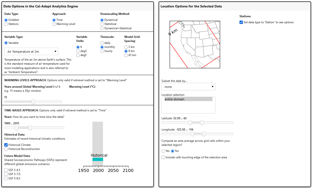
This allows a user to interactively select the various attributes to refine the datasets. Logic is built into the menu to filter out implausible combinations. Users can filter on time period, simulation(s), and spatially using the built-in geographies. Selected data can then be retrieved using:
data_to_use = selections.retrieve()Accessing Zarr data directly using QGIS 3.40.10+
The free and open source Geographical Information System software package QGIS can open Zarr stores stored in S3 directly. The 3.40.10 version of QGIS or later is required for this functionality. Note that this option only works for smaller files such as aggregated monthly data, GWL, or climate indices. QGIS can only access datasets with a limited number of raster bands, so hourly or daily data have too many bands to load successfully.
Best Use
Loading Analytics Engine Zarrs directly from S3 should be limited to datasets represented by warming level (as with the example below) or with a monthly time frequency. Daily or hourly datasets have too many bands to be loaded directly into QGIS.
Limitations
GDAL, which underpins QGIS, has a default limit of 65,000 bands for reading raster layers. This is to prevent excess memory consumption. This makes it not possible to load hourly or daily data, as the QGIS driver does not allow spatial or temporal filtering upon definition of the data connection.
Example Usage
To open the S3 Zarr store go to the menu item Layer→Add Layer→Add Raster Layer. This will bring up the Data Source Manager | Raster interface. Under Source Type switch the radio button to Protocol: HTTP(S), cloud, etc. then under the Protocol section choose AWS S3 for the Type, cadcat for the Bucket or container, and then enter the relative path to the Zarr store, which can be found by using the AWS Explorer or Data Catalog.. As an example to load the multi-model mean extreme heat absolute Zarr store, which is stored at various warming levels enter “tmp/era/wrf/cae/mm4mean/ssp370/gwl/TX99p/d03/” for Object Key.
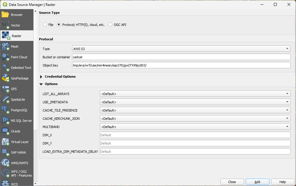
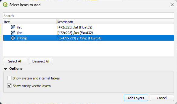
Clicking the Add button will bring up another menu. Select the variable name, in this case, TX99p. The shape of the array can be seen in the description with 472 by 223 spatial cells and 5 warming level bands.
This dataset is in Lambert Conformal projection used by WRF data. Here is the proj4 description of the custom projection:
+proj=lcc +lat_0=38 +lon_0=-70 +lat_1=30 +lat_2=60 +x_0=0 +y_0=0 +R=6370000 +units=m +no_defs +type=crsAnd the WKT projection definition:
PROJCRS["undefined",
    BASEGEOGCRS["undefined",
        DATUM["undefined",
            ELLIPSOID["undefined",6370000,0,
                LENGTHUNIT["metre",1,
                    ID["EPSG",9001]]]],
        PRIMEM["Greenwich",0,
            ANGLEUNIT["degree",0.0174532925199433],
            ID["EPSG",8901]]],
    CONVERSION["unnamed",
        METHOD["Lambert Conic Conformal (2SP)",
            ID["EPSG",9802]],
        PARAMETER["Latitude of 1st standard parallel",30,
            ANGLEUNIT["degree",0.0174532925199433],
            ID["EPSG",8823]],
        PARAMETER["Latitude of 2nd standard parallel",60,
            ANGLEUNIT["degree",0.0174532925199433],
            ID["EPSG",8824]],
        PARAMETER["Latitude of false origin",38,
            ANGLEUNIT["degree",0.0174532925199433],
            ID["EPSG",8821]],
        PARAMETER["Longitude of false origin",-70,
            ANGLEUNIT["degree",0.0174532925199433],
            ID["EPSG",8822]],
        PARAMETER["Easting at false origin",0,
            LENGTHUNIT["metre",1],
            ID["EPSG",8826]],
        PARAMETER["Northing at false origin",0,
            LENGTHUNIT["metre",1],
            ID["EPSG",8827]]],
    CS[Cartesian,2],
        AXIS["easting",east,
            ORDER[1],
            LENGTHUNIT["metre",1,
                ID["EPSG",9001]]],
        AXIS["northing",north,
            ORDER[2],
            LENGTHUNIT["metre",1,
                ID["EPSG",9001]]]]
LOCA2 data is loaded in WGS84 (EPSG:4326), which is automatically handled by QGIS.
By default, QGIS will symbolize the Zarr as a Multiband Color raster with the first 3 GWLs as bands. Double-click on the raster layer in the Layers pane to bring up the Symbology menu, then switch Render Type to Singleband pseudocolor. Then pick the band which represents the GWL of interest and hit Ok.
Downloading LOCA2 NetCDF data using the Cal-Adapt Data Download Tool
The Cal-Adapt Data Download Tool (DDT) allows users to easily download data packages of LOCA2 data, specifically the data in loca2/aaa-ca-hybrid. These data packages are pre-made groups or clusters of statistically downscaled LOCA2 data that are most commonly accessed on Cal-Adapt, which helps make data selection and download more intuitive and user-friendly.
Best Use
Downloading LOCA2 NetCDF data in bulk with the ability to temporally aggregate (Monthly) and spatially filter by county. Can download multiple scenarios, models, and metrics (variables) at once.
Limitations
Currently limited to the LOCA2 NetCDF datasets only. In addition, currently users are required to spatially filter by one or more counties, so they can not easily get the entire spatial extent of the data.
Example Usage
- Navigate to the Data Download Tool:
- Click the “Customize and Download” button under the data package of choice.
- Make custom selections in the “Review Your Data Package” sidebar including what frequency, which models, variables, and counties the user is interested in downloading.
- Click “Download Your Data” to create the data packages which are ready for download to a local machine.
Downloading LOCA2 NetCDF data using the AWS Explorer web page
Anyone can utilize existing AWS explorer functions within the Cal-Adapt: Analytics Engine S3 bucket to explore and download existing data through a web browser. Data can be accessed by navigating the file structure to identify and download NetCDF files to a local computer. This solution does not require an Analytics Engine login and does not require coding.
Best Use
Since web browsers only allow download of individual files rather than whole directory structures, the AWS Explorer is best used only for downloading NetCDF files in loca2/aaa-ca-hybrid, and in this capacity, it would be better to use the AWS CLI toolset for downloading more than a few files.
Limitations
Can only download files separately and does not preserve the directory structure they are housed in S3.