Model Uncertainty
What is model uncertainty?
Global climate models (GCMs) are complex mathematical representations of Earth’s atmosphere, ocean, land surface, and sea ice, designed to simulate the physical processes that govern climate. Because no single model can perfectly capture the full complexity of the climate system, researchers have long recognized the value of using multiple models. Multi-model ensembles are collections of simulations from different modeling centers around the world. They allow scientists to sample a broader range of structural assumptions, parameterization schemes, and numerical approaches, providing a more robust picture of both the mean climate state and its uncertainty.
The use of multi-model data has become a cornerstone of modern climate science, most notably through coordinated international efforts like the Coupled Model Intercomparison Project (CMIP). By comparing and combining outputs from dozens of independently developed models, researchers can identify areas of strong agreement, which boosts confidence in projected outcomes, as well as areas of divergence, which highlight key uncertainties. This approach not only improves the reliability of global projections but also underpins the assessment reports of the Intergovernmental Panel on Climate Change (IPCC), making multi-model analysis essential for translating climate science into actionable policy guidance.
Beyond capturing uncertainty, using multiple models also takes advantage of the fact that no single model excels at everything. Individual GCMs are not interchangeable, each one tends to capture certain regional climates, atmospheric dynamics, or feedback processes more faithfully than others. Different models are developed with different priorities and strengths, some better reproduce large-scale atmospheric circulation patterns, others more accurately simulate regional precipitation or land-surface feedbacks, and still others are optimized for ocean-atmosphere coupling. When models are pooled together, their complementary strengths combine to produce a more complete picture of the climate system than any individual model could provide on its own. This is a compelling practical reason to embrace a multi-model approach: rather than betting on one “best” model, you benefit from the collective capability of the ensemble. For users communicating with decision-makers, this is a practical and intuitive justification for multi-model analysis: using a single model would mean betting on one team of scientists being right about everything, whereas using an ensemble means drawing on the best available understanding from research groups around the world, each with different methodological strengths.
Model uncertainty reflects the fact that different modeling groups make different scientific choices about how to represent complex climate processes. Each model is a legitimate tool built on valid physical principles; the spread between them captures the range of outcomes that current science considers plausible. The appropriate response is to characterize that range honestly, communicate it clearly, and design decisions that are robust across it.
“Sound decision-making that anticipates, prepares for, and responds to climate change depends on information about the full range of possible consequences and associated probabilities… Low-probability outcomes can have significant impacts, particularly when characterized by large magnitude, long persistence, broad prevalence, and/or irreversibility.”1
What CMIP6 models are used in these analyses?
All analyses on this page use monthly near-surface air temperature, tas and precipitation, pr from the CMIP6 archive for models that provide both a historical simulation (1850–2014) and a future simulation under SSP3-7.0. Data are subsetted to California and expressed as anomalies relative to the 1850–1900 pre-industrial baseline, placing results directly in the global warming levels (GWL) framework used by the IPCC AR6.
Within the broader CMIP6 archive, the Cal-Adapt Analytics Engine uses a curated subset of eight models that meet bias-adjustment criteria and provide output at sufficient spatial resolution for California impact assessments: FGOALS-g3, EC-Earth3-Veg, CESM2, CNRM-ESM2-1, MIROC6, MPI-ESM1-2-HR, EC-Earth3, and TaiESM1. Analyses on this page show results for both the full available CMIP6 archive and this Analytics Engine subset, so users can see how the curated eight compare to the broader distribution.
How does model uncertainty change over time?
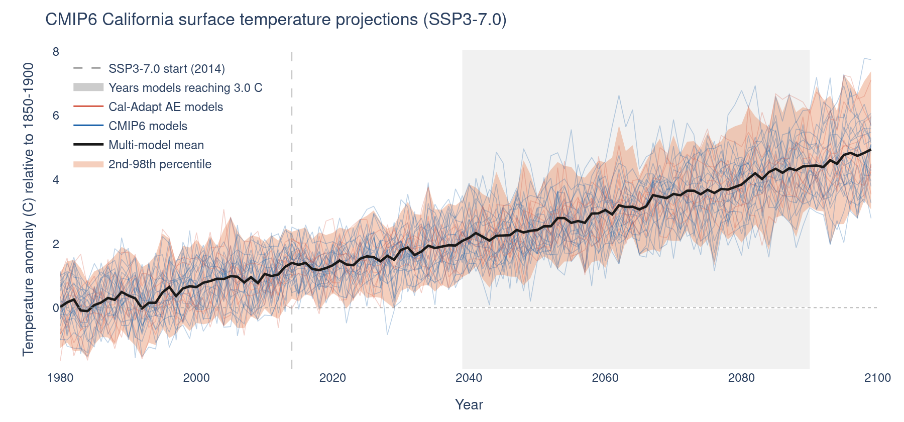
A few things are worth noting when reading Figure 1:
The spread grows with time. In the historical period (before 2015), model traces are tightly clustered because all models are trained on the same observed climate before 2015. After 2015, the traces fan out as both scenario and model differences compound. By end of century, the range between the warmest and coolest models for California can exceed 3–4°C, a difference that is highly consequential for planning.
The warming-level band. The grey shaded vertical band marks the range of calendar years in which different models reach the selected global warming level (e.g., 3°C above pre-industrial). Fast-warming models reach it decades earlier than slow-warming models. This spread in timing is itself a form of model uncertainty (in the global climate sensitivity) and it means that time-based analyses (e.g., “mid-century”) mix models at very different stages of their warming trajectories. The global warming levels framework avoids this problem by anchoring comparisons to physically comparable climate states rather than calendar years.
The multi-model mean is not a best estimate. The multi-model mean (MMM) is a useful summary of the ensemble’s central tendency, and in hindcast evaluations it often outperforms any individual model. However, treating the MMM as a best estimate in a planning context is inappropriate for two reasons:
First, it can mask bimodal distributions, where models cluster in two groups with qualitatively different outcomes and the mean falls between them. A closer look at the individual model traces reveals that the ensemble is not uniformly distributed, with a small number of models (e.g. CanESM5, EC-Earth3-Veg) project end-of-century anomalies of 7–8°C, well above the main cluster of models which converge between 3–5°C. This separation illustrates the bimodal behavior described above: the multi-model mean of ~4.7°C falls between these two groups, potentially misrepresenting both. Users relying solely on the MMM would miss the possibility of these high-end outcomes entirely.
Second, and more fundamentally, it discards the range, which is often the most important information for risk-based decisions. The IPCC guidance is explicit: information on the tails of the distribution should always be reported alongside any central estimate.
What does the spread look like by the end of century?
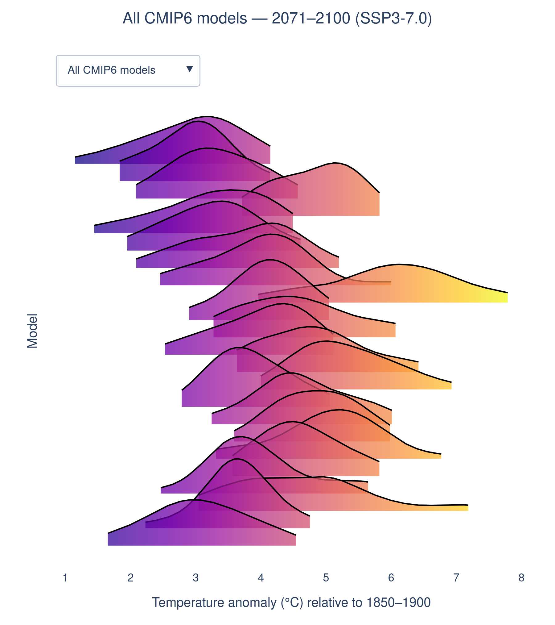
Figure 2 shifts from a temporal view to a distributional one. Each ridge shows what one model’s range of outcomes looks like by the end of century. Two key features to note:
- Within-model spread: Ridge width shows how much year-to-year variability a given model produces within the period. Wide ridges indicate high internal variability in that model’s simulation.
- Between-models spread: Offset of medians between ridges reflects the structural model uncertainty.
How does the specific location influence the model uncertainty?
Warming Levels denote what is the Global Warming around the world, and the models show what is the regional amount of warming felt in X area when global warming reaches Y warming level. This means that the same warming level can correspond to different regional warming across models and regions, which is a direct manifestation of structural model uncertainty. To illustrate this, in Figure 3 we can look at the distribution of temperature anomalies at the end of century for each California sub-region (Coastal CA, Southern CA, Sierra Nevada) at the selected global warming levels of 1.5°C, 2°C, and 3°C (controlled by the warming level toggle selector), while the x-axis shows the range of temperature anomalies projected by each model for that region at that warming level. Each dot represents one model’s projection for that region and warming level; the diamond marks the multi-model mean; the shaded rectangle spans the full range of model projections.
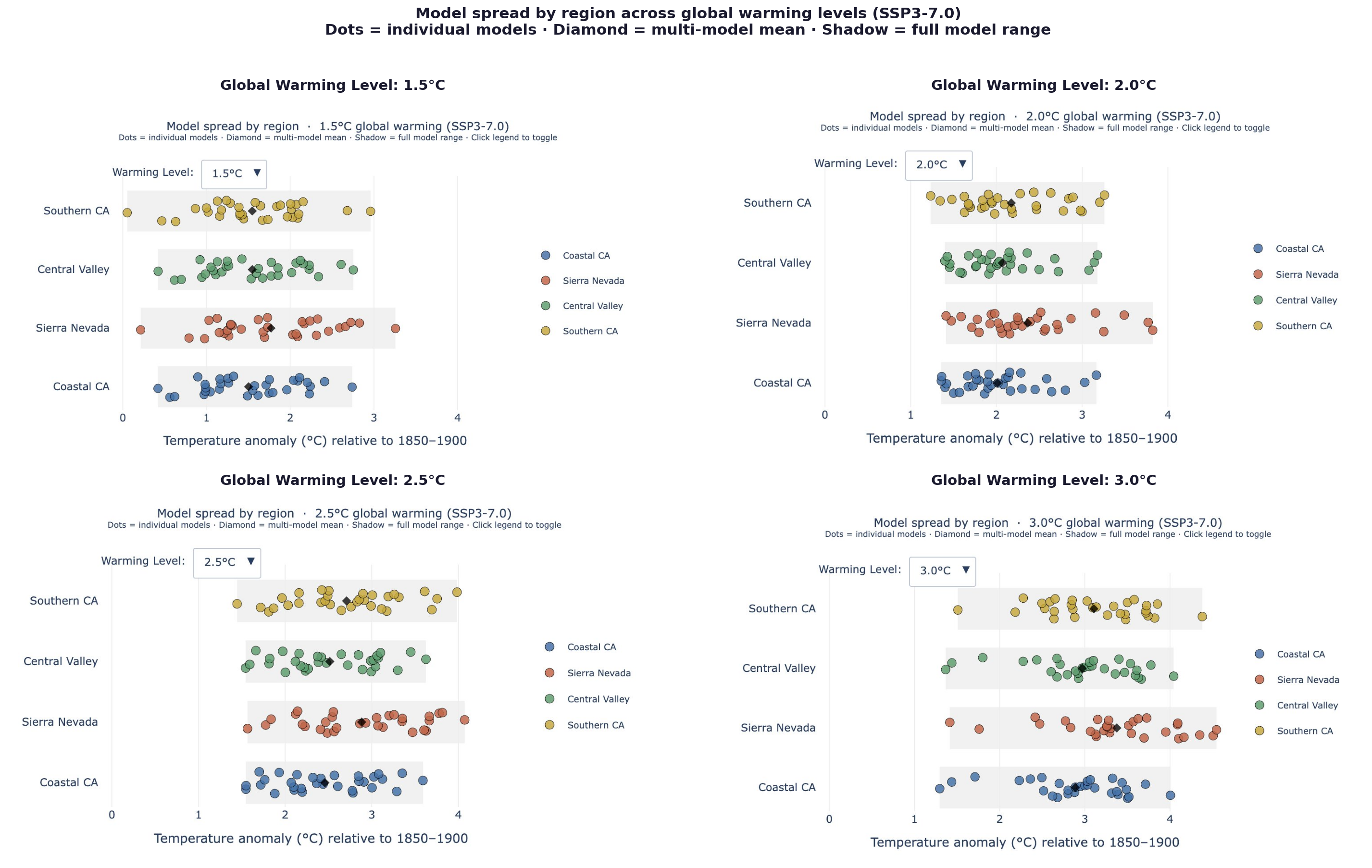
As shown in Figure 3, the entire distribution shifts right from 1.5°C to 3.0°C, as expected. But the shift is not uniform across regions or models:
- Southern CA and Sierra Nevada consistently show the widest spread: the grey shadow is notably longer for these regions than for Coastal CA. This means model choice has a larger absolute impact on exposure estimates in these regions. For water supply and fire risk assessments in the Sierra Nevada, the difference between the warmest and coolest models can exceed 2°C at 3.0°C GWL.
- Coastal CA has the tightest model agreement, possibly meaning that the ocean moderates the warming signal and inter-model spread. The spread grows with warming level: at 1.5°C the distributions are relatively compact; by 3.0°C they fan out considerably. This is the visual demonstration that structural model uncertainty compounds over time and with forcing level.
- Some models are consistently outliers: looking across panels, the leftmost and rightmost dots in each region tend to be the same models across warming levels. This suggests some models are systematically cooler or warmer for California regardless of the warming level, which reflects persistent differences in regional climate sensitivity across model families.
- The MMM shifts right faster in interior regions: comparing the diamond position relative to the x-axis across regions, Southern CA and Sierra Nevada warm faster than Coastal CA per degree of global warming.
Relationship between warming rate and end-of-century anomaly
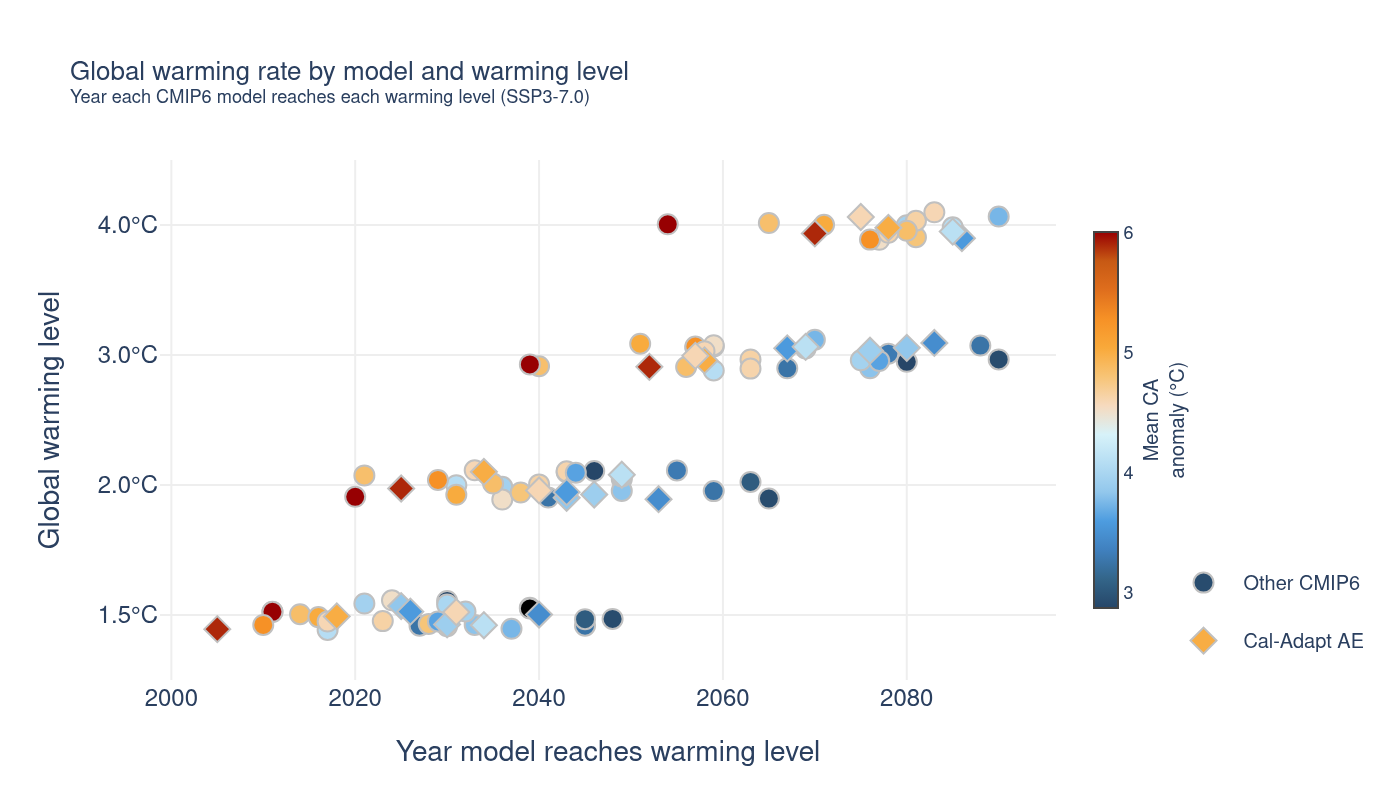
As shown in Figure 4, there is not a definite correlation between end-of-century temperature anomaly and the year a model reaches a given warming level. You might expect that a model reaching, say, 3°C in California earlier would also project higher end-of-century California temperatures, but the scatter shows this is not consistently the case. A model can warm California quickly to a threshold and then level off, or warm it slowly but continue accelerating late in the century.
This suggests that the rate at which California reaches a warming level is not a reliable predictor of where it ends up by 2100, as the two are driven by partially independent aspects of each model’s behavior (early forcing response vs. late-century trajectory).
This is a manifestation of structural model uncertainty: different models have different sensitivities and feedbacks that govern their warming trajectories, and these differences do not necessarily align with global warming rates.
Are all climate variables equally variable across models?
No. Model uncertainty varies substantially across variables.
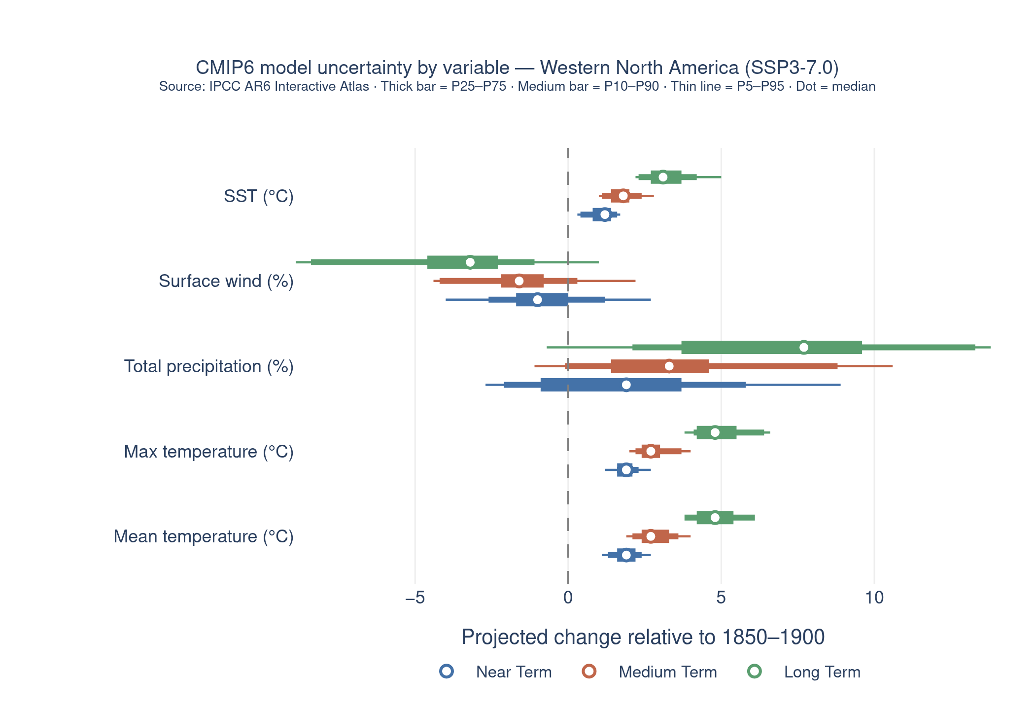
Figure 5 shows CMIP6 model uncertainty for five climate variables in Western North America under SSP3-7.0, across three time horizons.
High confidence, robust signal. Mean temperature, max temperature, and SST all show tight distributions that sit entirely to the right of zero across all three periods. The IQR (thick bar) is narrow relative to the median, and all models agree on the direction of change, warming is virtually certain. The spread grows modestly from near-term to long-term, but remains well-constrained. This supports high confidence in both the direction and approximate magnitude of warming.
Low confidence, sign uncertainty. Total precipitation has by far the widest distribution of any variable. At all three time horizons the P5–P95 whisker crosses zero, meaning some models project drying while others project wetting. The long-term median is positive (~+8%) but the lower tail extends below zero (-0.7% at P5), confirming that even by end of century the direction of change is not robust across the full ensemble. The spread is disproportionately large relative to the median signal.
Moderate spread, consistent slowing signal. Wind shows a consistent negative signal (decreasing surface wind speeds) across all periods, with the long-term distribution entirely below zero at the P25–P75 level. However, the P5–P95 range crosses zero for near- and medium-term periods, indicating lower confidence at shorter horizons. By the long term, confidence in the direction increases.
The contrast grows over time: For temperature variables, the distributions shift right and remain tight and the signal-to-noise ratio improves with time. For precipitation, the distributions widen substantially from near-term to long-term without a proportional increase in the median, uncertainty accumulates faster than the signal strengthens.
How should users communicate uncertainty in their analyses?
The IPCC AR5 guidance framework1 offers two calibrated metrics for communicating certainty in climate findings:
- Confidence (qualitative): synthesizes the type, amount, quality, and consistency of evidence and the degree of agreement among models and studies. Expressed as very low, low, medium, high, or very high.
- Likelihood (quantitative): expresses a probabilistic estimate of an outcome. Expressed using calibrated language such as virtually certain (99–100%), very likely (90–100%), likely (66–100%), about as likely as not (33–66%), unlikely (0–33%).
Users should report these distinctions explicitly, rather than presenting the multi-model mean alone. Where confidence is low — particularly for precipitation — it is important to explain why confidence is low (model disagreement on direction, not data limitations) and to present the full range rather than a single number.
- For temperature-driven questions: the MMM is a defensible central estimate; the 10th–90th percentile envelope captures the planning range.
- For precipitation-driven questions: always use the full model ensemble; the MMM alone discards critical information about sign uncertainty.
- For compound questions (heat and drought, heat and flood): preserve the full joint distribution of temperature and precipitation across models; do not select on either variable independently.
Key takeaways
- Model uncertainty represents genuine scientific disagreement about climate system behavior. It is a property of the science, not a limitation of the Analytics Engine tools.
- For California temperature, model uncertainty is relatively well-characterized: models agree on the direction of change with high confidence, and the multi-model mean is a useful summary when accompanied by the ensemble range.
- For California precipitation, model uncertainty is large enough that models often disagree on the direction of change. In these cases, the multi-model mean can be misleading, and the full ensemble range is essential.
- Model uncertainty is not uniform, it varies by variable, region, and time horizon, and treating it as a single problem leads to unreliable decisions.
- The spread between models grows over time. Planning for longer time horizons requires engaging with a wider range of possible futures, not narrowing to a single projection.
- Uncertainty should be communicated using calibrated language consistent with IPCC practice: confidence levels for qualitative assessments and likelihood language for probabilistic ones. Reporting only the multi-model mean without the range does not meet this standard.